|
OpenMS
|
The following sections explain the example pipelines TOPPAS comes with.
You can open all examples pipelines by selecting File > Open example file in TOPPAS.
All input files and parameters are already specified, so you can just hit Pipeline > Run (or press F5) and see what happens.
The file peakpicker_tutorial.toppas can be inspect it in TOPPAS via File -> Open example file. It contains a simple pipeline representing a common use case: starting with profile data, the noise is eliminated and the baseline is subtracted. Then, PeakPickerHiRes is used to find all peaks in the noise-filtered and baseline-reduced profile data.

This section describes an example identification pipeline contained in the example directory, Ecoli_Identification.toppas. Inspect it in TOPPAS via File -> Open example file. It is shipped together with a reduced example mzML file containing 139 MS2 spectra from an E. coli run on an Orbitrap instrument as well as an E. coli target-decoy database (which was created using DecoyDatabase).
We use the search engine Comet (Eng et al., 2012) for peptide identification. Therefore, Comet must be installed and the path to the Comet executable (Comet.exe) must be set in the parameters of the CometAdapter node. If you installed OpenMS using our binary-package installers, chances are, Comet is already available on your system and in your $PATH environment variable, and the adapter will just work out of the box.

Extensions to this pipeline would be to do the annotation of the spectra with multiple search engines and combine the results afterwards, using the ConsensusID TOPP tool.
The results may be exported using the TextExporter tool, for further downstream analysis with non-OpenMS tools.
The simple pipeline described in this section (BSA_Quantitation.toppas) can be used to quantify peptides that occur on different runs (you can inspect it in TOPPAS via File -> Open example file). The example dataset contains three different bovine serum albumin (BSA) runs. First, FeatureFinderCentroided is called since the dataset is already centroided (i.e. peak picking took place already). The results of the feature finding are then annotated with (existing) identification results. For convenience, we provide these search results (as idXML files) with an FDR of 5% in the BSA directory.

Identifications are mapped to features (3D quantitation points of peptide signals) by the IDMapper. The last step is performed by FeatureLinkerUnlabeled which links corresponding features across runs. The results can be used to calculate ratios, for example. The data could also be exported to a text based format using the TextExporter for further processing (e.g., in Microsoft Excel).
The results can be opened in TOPPView. The next figures show the results in 2D and 3D view, together with the feature intermediate results. One can see that the intensities and retention times are slightly different between the runs. To correct for retention times shift, a map alignment could be done, either on the spectral data or on the feature data.


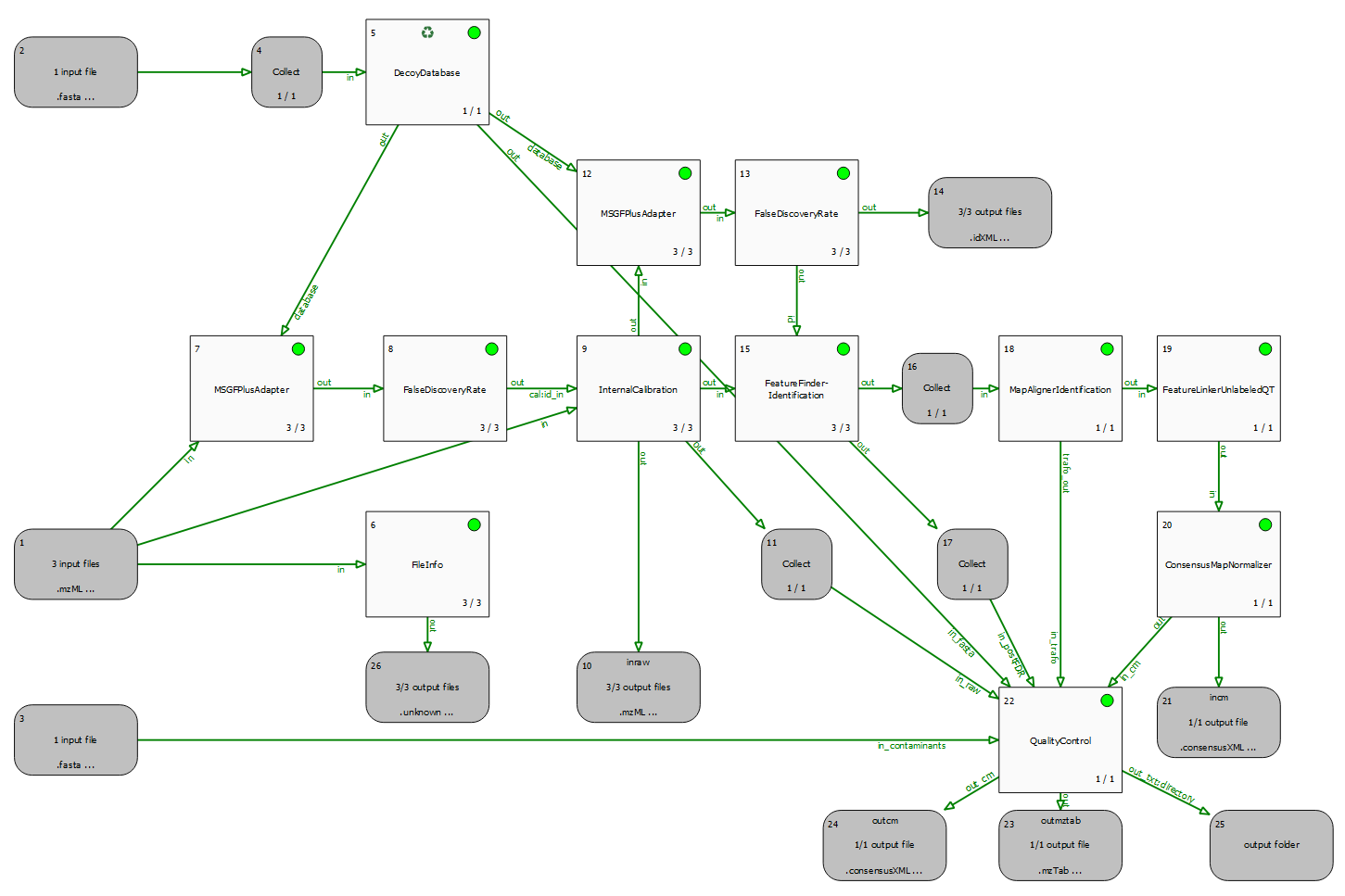
A quality control pipeline for DDA data (QualityControl.toppas), which also performs identification (using MSGFPlusAdapter), mass calibration (using InternalCalibration) and quantitation (using FeatureFinderIdentification).
Since we analyse more than one raw file (run), we can also employ MapAlignment and FeatureLinking, to transfer identifications and enable a quantitative comparison across samples.
Finally, the QualityControl node receives all intermediate and final output data to extract and compute quality metrics. These are exported in the form several output files which can be inspected.
Most important is probably the output folder (node #25), which contains MaxQuant compatible output (evidence.txt and msms.txt). These .txt files can be used as input to external tools, such as PTX-QC to automatically obtain a comprehensive QC report.
We will use a special FDR search strategy described by Lin et al.. It uses a mode of DecoyDatabase which allows to create a special "neighbor" database to control the FDR.
The example pipeline is named FDR_NeighborSearch.toppas. Inspect it in TOPPAS via File -> Open example file. A description is provided within the TOPPAS workflow.
The following example is actually not a useful workflow but is supposed to demonstrate how merger and collector nodes can be used in a pipeline. Have a look at merger_tutorial.toppas. Inspect it in TOPPAS via File -> Open example file.

In short: mergers require multiple input edges, whose data is combined bit by bit. Collectors on the other hand usually only have one input edge and combine all files from this single edge into a list in one go. The succeeding tool will be invoked only once, with a list of input files.
In detail, a merger merges its incoming file lists, i.e., files of all incoming edges are combined into new lists. Each file list has an many elements as the merger has incoming connections. And there are as many lists as there are files(rounds) from the the preceeding(=upstream) tool. The tool downstream of the merger is invoked with these merged lists as input files. All incoming connections should pass the same number of files (unless one of the upstream nodes is in "recycling mode"), such that all merged lists have the same number of files. In other words, if you have K input edges with N files each, the merger will create N output lists, with K elements each.
A collector node, on the other hand, waits for all rounds to finish on its upstream side before concatenating all files from all incoming connections into one single list. It then calls the next tool with this list of files as input. This will happen exactly once during the entire pipeline run.
In order to track what is happening, you can just open the example file and run it. When the pipeline execution has finished, have a look at all input and output files (e.g., select Open in TOPPView in the context menu of the input/output nodes). The input files are named rt_1.mzML, rt_2.mzML, ... and each contains a single spectrum with RT as indicated by the filename, so you can easily see which files have been merged together.
 1.9.8
1.9.8 